Standard Bayesian Optimization with FCVOpt

While FCVOpt is designed for hyperparameter optimization via fractional cross-validation, the underlying BayesOpt class can be used for standard Bayesian optimization of any black-box function—no cross-validation required.

This notebook demonstrates BayesOpt on the classic Branin function, a standard benchmark for global optimization. Unlike the CV setting, the observed objective values here are direct evaluations of the true loss function (not fold-level proxies), so we can meaningfully plot the best observed value so far and track how the optimizer converges to the global minimum.

The Branin Function

The 2-dimensional Branin function is defined as:

\[f(x_1, x_2) = a\left(x_2 - bx_1^2 + cx_1 - r\right)^2 + s(1-t)\cos(x_1) + s\]

with standard constants \(a=1\), \(b=5.1/(4\pi^2)\), \(c=5/\pi\), \(r=6\), \(s=10\), \(t=1/(8\pi)\), over the domain \(x_1 \in [-5, 10]\), \(x_2 \in [0, 15]\).

It has three global minima, all attaining \(f^* \approx 0.3979\):

• \((-\pi,\; 12.275)\)

• \((\pi,\; 2.275)\)

• \((9.425,\; 2.475)\)

import numpy as np
import matplotlib.pyplot as plt

from fcvopt.optimizers import BayesOpt
from fcvopt.configspace import ConfigurationSpace
from ConfigSpace import Float

Define the Objective Function

BayesOpt expects an objective that takes a dict of hyperparameter values and returns a scalar. We wrap the Branin formula accordingly.

def branin(params: dict) -> float:
    """Branin function. Global minimum f* ≈ 0.3979."""
    x1, x2 = params['x1'], params['x2']
    a, b, c = 1.0, 5.1 / (4 * np.pi**2), 5.0 / np.pi
    r, s, t = 6.0, 10.0, 1.0 / (8 * np.pi)
    return float(a * (x2 - b * x1**2 + c * x1 - r)**2 + s * (1 - t) * np.cos(x1) + s)

BRANIN_OPTIMUM = 0.397887
print(f"Branin global minimum: {BRANIN_OPTIMUM:.6f}")
print(f"Value at (pi, 2.275): {branin({'x1': np.pi, 'x2': 2.275}):.6f}")

Branin global minimum: 0.397887
Value at (pi, 2.275): 0.397887

Define the Search Space

We use FCVOpt’s ConfigurationSpace to declare the two continuous inputs with their standard Branin bounds.

config = ConfigurationSpace(seed=42)
config.add([
    Float('x1', bounds=(-5.0, 10.0)),
    Float('x2', bounds=(0.0, 15.0)),
])
print(config)

Configuration space object:
  Hyperparameters:
    x1, Type: UniformFloat, Range: [-5.0, 10.0], Default: 2.5
    x2, Type: UniformFloat, Range: [0.0, 15.0], Default: 7.5

Run Standard Bayesian Optimization

BayesOpt follows the same API as FCVOpt but fits a standard (non-hierarchical) GP directly on the observed (x, y) pairs.

Key arguments:

Argument	Description
obj	Black-box function: dict → float
config	Hyperparameter / input search space
acq_function	'EI' (Expected Improvement), 'LCB', or 'KG'
tracking_dir	Local directory for MLflow experiment logs
experiment	MLflow experiment name
seed	Random seed for reproducibility

We run 30 total evaluations: 5 random initializations followed by 25 acquisition-guided steps.

optimizer = BayesOpt(
    obj=branin,
    config=config,
    acq_function='EI',
    tracking_dir='./opt_runs/',
    experiment='branin_standard_bo',
    seed=123,
)

best_conf = optimizer.optimize(n_trials=30, n_init=5)
optimizer.end_run()

Number of candidates evaluated.....: 30
Observed obj at incumbent..........: 0.398315
Estimated obj at incumbent.........: 0.423703

 Best Configuration at termination:
 Configuration(values={
  'x1': 9.4327962845392,
  'x2': 2.4926768337029,
})

print(f"Best configuration found:")
print(f"  x1 = {dict(best_conf)['x1']:.4f}")
print(f"  x2 = {dict(best_conf)['x2']:.4f}")
print(f"  f(x1, x2) = {branin(dict(best_conf)):.6f}")
print(f"  Known global minimum = {BRANIN_OPTIMUM:.6f}")
print(f"  Optimality gap = {branin(dict(best_conf)) - BRANIN_OPTIMUM:.6f}")

Best configuration found:
  x1 = 9.4328
  x2 = 2.4927
  f(x1, x2) = 0.398315
  Known global minimum = 0.397887
  Optimality gap = 0.000428

Optimization Progress

Internally, BayesOpt selects the incumbent at each step as the training point with the lowest GP posterior mean—not necessarily the lowest observed value. This means f_inc_obs (the observed value at the GP-based incumbent) can fluctuate non-monotonically as the GP model is updated.

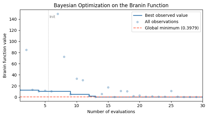
Because we are optimizing a direct, noise-free function rather than a CV proxy, a cleaner quantity to track is the best observed value so far: the running minimum over all evaluations. This is guaranteed to decrease monotonically and directly reflects how much the optimizer has improved the objective.

The plot below shows this quantity alongside all individual observations, with the known global minimum as a dashed reference line.

observed_y = optimizer.observed_values
best_so_far = np.minimum.accumulate(observed_y)
n_evals = np.arange(1, len(observed_y) + 1)

fig, ax = plt.subplots(figsize=(7, 4))

ax.step(n_evals, best_so_far, where='post', color='steelblue', lw=2, label='Best observed value')
ax.scatter(n_evals, observed_y, color='steelblue', alpha=0.35, s=20, zorder=3, label='All observations')
ax.axhline(BRANIN_OPTIMUM, color='tomato', lw=1.5, ls='--', label=f'Global minimum ({BRANIN_OPTIMUM:.4f})')
ax.axvline(5.5, color='gray', lw=1, ls=':', alpha=0.7)
ax.text(5.7, observed_y.max() * 0.95, 'Init', color='gray', fontsize=9)

ax.set_xlabel('Number of evaluations')
ax.set_ylabel('Branin function value')
ax.set_title('Bayesian Optimization on the Branin Function')
ax.legend(loc='upper right')
ax.set_xlim(1, len(observed_y))
plt.tight_layout()
plt.show()